Chiarella Calibration Tutorial

This model simulates a synthetic financial market and is based on the Extended Chiarella Model, described in the following publication:

Majewski, A. A., Ciliberti, S., & Bouchaud, J. P. (2020). Co-existence of trend and value in financial markets: Estimating an extended Chiarella model. Journal of Economic Dynamics and Control, 112, 103791.)

Here we present an implementation of this model in the Simudyne SDK.

Download Model Files

The code for this model is available as a zip download, containing a complete model as a Maven project. This project should be able to be run from Maven or any Java IDE environment.

Abstract (from original paper)

Trend and Value are pervasive anomalies, common to all financial markets. We address the problem of their co-existence and interaction within the framework of Heterogeneous Agent Based Models (HABM). More specifically, we extend the Chiarella (1992) model by adding noise traders and a non-linear demand of fundamentalists. We use Bayesian filtering techniques to estimate the model on monthly time series of prices across a variety of asset classes since 1800. The fundamental value is an output of the estimation, and does not require the use of an external pricing model. Our extended model reproduces many empirical observations, including the non-monotonic relation between past trends and future returns. The destabilizing activity of trend-followers leads to a qualitative change of mispricing distribution, from unimodal to bimodal, meaning that some markets tend to be over- (or under-) valued for long periods of time.

Model overview

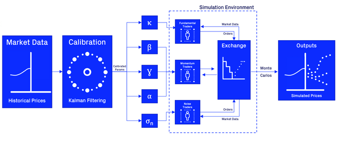
This model simulates a synthetic market, including all relevant contributing participants. This simulation is set up to model the price changes of an asset. These price dynamics are caused by the actions of the contributing agents. In a nutshell, this model contains trader agents and an exchange agent.

The traders submit buy and sell orders on each step. The exchange calculates the overall demand and supply from the cumulative buy and sell orders, based on which the asset price is updated. This updated price is then fed back to the traders so that they can adjust their behavior in the next step.

The market shows evolving price dynamics based on this recurrent interaction and the specified trading strategies. Changes in the specific contribution of different trading strategies will affect the behavior of the simulated market.

Agents & Network

There are 4 types of agents in this model: (1) an Exchange agent, (2) three different types of trader agents.

The three kind of traders in this model differ in their strategies based on what they decide to buy or sell:

1. Fundamental traders base their investments on the perceived intrinsic (or fundamental) value of the asset. A fundamental trader will buy an asset whenever it is underpriced, according to her beliefs, and otherwise she will sell.
2. Momentum traders use a trend (or momentum) signal, which indicates the recent change in prices. This signal indicates whether the price has changed in upwards or downwards direction.
3. Noise traders represent traders who either have different investment horizon than we are considering (months) or are following investment strategies different than trend-following or value investing strategy. Their behavioral choices are implemented as random choices. This group of traders contributes price volatility that can not be explained by either fundamental value or momentum.

Exchange

The exchange aggregates all buy and sell orders and updates the asset price accordingly. In this model, it is assumed that the price dynamics is governed by a linear price impact mechanism: the price change from t to t + ∆ is linear in the cumulative demand imbalance (total net demand: demand - supply) in the same period, which we denote as D (t, t + ∆). This can be written as

P(t+∆) − P(t) = λD(t, t+∆)

where λ is ‘Kyle’s lambda’ which is assumed to be inversely proportional to the liquidity of the market in real-world scenarios. λ is used as weighting parameter to control the influence of supply and demand on the price. Specifically, λ is a linear approximation of the market impact we would observed on the buy and sell limit orderbooks as traders submits limit and market orders.

Traders

The aggregated demand depends on the investment strategies of market participants, which we assume are heterogeneous in their investment decisions (as explained above). The total demand of all three trader types is given by the following equation:

Equation 3.2 from paper

whereby the total demand is a combination of the demand of fundamental traders (first component) weighted by κ, the demand of momentum traders (second component) weighted by β, and the noise trader influence (last component) weighted by σ_N. The parameters κ, β, σ_N are therefore a way of tuning the overall influence of each trader group on the total demand.

Fundamental traders

As explained above, fundamental traders will buy and sell based on a discrepancy between a perceived fundamental Value (Vt) and the market price (Pt), whereby the fundamental trader buys if there an asset is underpriced (Vt - Pt > 0). The demand is directly proportional to the price distortion, i.e. fundamental traders will place larger buy or sell orders if an asset is heavily under- or over-priced. The fundamental value Vt is assumed to be driven by a diffusion process with volatility σV and average growth g:

dV(t) ~ N(g , σ_V)

Since the overall demand of all fundamental traders is controlled by the parameter κ, each individual traders demand is scaled by:

κ_i = $\frac{κ}{number \ of \ fundamental \ traders}$

Momentum traders

Momentum traders calculate a trend signal as an exponentially moving average over recent changes in the price, M(t). Here, a decay rate α scales the influence of past versus recent changes in market price. The current momentum is hereby calculated as follows:

M(t) = α * (P(t) - P(t-1)) + (1 - α) * M(t-1)

The total demand of momentum traders is derived by the function:

β * tanh(γ * M(t))

indicating that the demand will increase with increased momentum, but will be bounded for extreme momentum values.

As for the fundamental traders, the overall demand of all momentum traders is controlled by the parameter β, therefore the demand for each single momentum trader is defined by:

β_i = $\frac{β}{number \ of \ momentum \ traders}$

Noise traders

Noise traders cover all other trading strategies that are not captured in the fundamental or momentum strategy. The cumulative demand of noise traders is described by Brownian Motion, with volatility σ_N, which describes the contribution of noise traders in the market.

Since σ_N controls the overall volatility induced by all noise traders, the individual contribution of each noise trader needs to decompose the overall volatility. To achieve this, each noise trader has a probability, p_order to engage with trading activities on a given step:

p_order = $\frac{1}{number \ of \ noise \ traders}$

If the trader decides to engage in trading activities on a given step, it randomly decides whether to buy or sell (50:50 chance).

This generates a trinomial lattice of a noise trader submitting a buy of volume +σ_N with a probability of $\frac{p_{order}}{2}$ and a sell of volume -σ_N with a probability $\frac{p_{order}}{2}$ of and a probability 1-p_order of doing nothing at each step, which converges to the Brownian Motion given in Equation 3.2 of the total demand of all noise traders.

Calibration

In this model, multiple parameters control the agents' behaviors and thus the overall model dynamics. In order to derive realistic model predictions, these parameters should be calibrated based on real-world data. This model is focused on predicting the price dynamics of an asset. Therefore, historic data of price changes can be used to estimate the hidden parameters (fitting parameters that have most likely produced the observed price changes). The changes in price of an asset can be described with the following equation:

Equation 3.7 from paper

Utilizing historic data and using optimization techniques such as an expectation maximization algorithm, we can find the model parameters that have most likely produced historic data, thus calibrating our model to existing data and ensuring that the agents behaviors are as realistic as possible. One of the main challenges for calibrating this model is the fact that the behavior of fundamental traders depends on the fundamental value signal, which itself is an unobserved (i.e. hidden) variable. However, it has been shown that this fundamental can be directly inferred from the observed price changes and thus can be jointly estimated with the model parameters.

After having conducted this calibration effort, the derived model parameters can be injected into the agent-based simulation, which enables to reproduce realistic price dynamics of an asset of interest.

Input parameters

After having conducted a calibration we can input the derived parameters in our model to closely resemble the price dynamics of an asset of interest. A list of all relevant parameters can be found below:

• Number of fundamental traders
• Number of momentum traders
• Number of noise traders
• Kyle's lambda controlling the impact of demand on price changes (λ)
• Initial fundamental value (V₀)
• Initial price distortion (V₀ - P₀)
• Initial momentum (M₀)
• Average drift of the fundamental value (g)
• Volatility of the fundamental value (σ_V)
• Influence of fundamental traders on the overall demand (κ)
• Decay rate for momentum calculation, i.e. horizon over which the momentum is calculated (α)
• Saturation factor with which momentum is mapped to demand (γ)
• Influence of momentum traders on the overall demand (β)
• Influence/volatility induced by noise traders (σ_N)

Model outputs

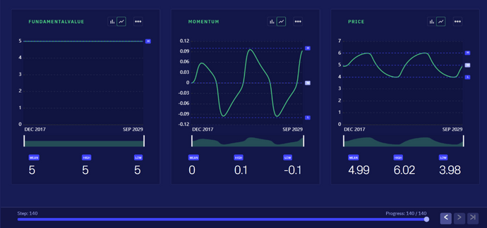
The figure below provides an example of a model simulation, showcasing the produced model outputs. As mentioned, the main focus of this model is the simulation of price dynamics. In order to understand the driving forces behind the observed price dynamics there are also outputs for the fundamental value signal, the momentum and overall demand.

In this example, we used the model to reproduce results from the original paper (Figure 2A&C of the Ciliberti et al. paper) where no noise traders are included and the model produces an oscillatory behavior based on the interaction between value and trend dynamics. Here, the momentum drives the price up until the asset is so overpriced that fundamental traders correct the price towards the fundamental value. This then creates negative momentum leading to an oscillation in the opposite direction. Through this mechanism of interaction between fundamental and momentum traders the prices oscillates periodically around the fundamental value.

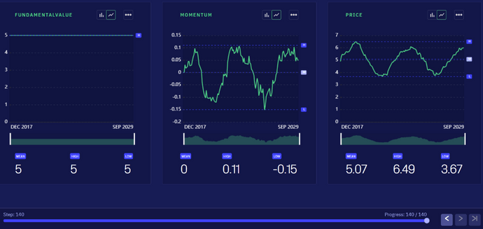
Now we will introduce noise traders into the system. Notice that we still see the oscillation in price however the signal has become noisier.