

CCP Risk Model
Last updated on 21st April 2026
Introduction
You can also find the original paper from Deloitte on their website: Agent-based modelling for central counterparty clearing risk | Deloitte UK
Central counterparties (CCPs) and clearing members (CM) are of crucial importance in enhancing the efficiency, stability and smooth trading of derivatives such as futures. CCPs are created to manage the overall credit risks of their respective CM’s by adopting a number of mitigants to ensure that they are nearly risk-free entities, such as the enforcement of margins and a default fund contribution from each CM. However, the assumption of CCPs being perceived as “risk-free” entities have been challenged following an adverse event that led to the default of a relatively small CM and subsequent depletion of two-thirds of the CCP’s default fund.
Existing models that are available to quantify the counterparty credit risk to a CCP are inadequate because it assumes that the behaviour of each CM is homogeneous: it fails to account for the potential for small CMs in taking on outsized and unhedged positions, which can introduce as much credit risk as all the other CM’s combined 1. This indirectly increases the credit risk of other CM’s because of the complex loss-sharing mechanisms that is adopted by the CCP (i.e. joint contribution of the default fund).
To overcome this limitation, an agent-based model (ABM) is developed to improve estimates of a CCP’s overall credit risk. This is achieved with a Monte Carlo simulation to quantify the severity of a default (and their probabilities) that is caused by a CM in the event of an external shock. The ABM model has various applications:
- It provides a tool for banks to quantify the counterparty credit risk to a CCP and make decisions on its own membership of the CCP; and
- Enables a CCP to test the effectiveness of various risk-mitigating procedures to keep the overall credit risk at a minimum.
Agents and Structure
The ABM consists of two main agent types: CMs (banking & non-banking) and the exchange/central counterparty (CCP). The network structure of the model is shown in the figure below.
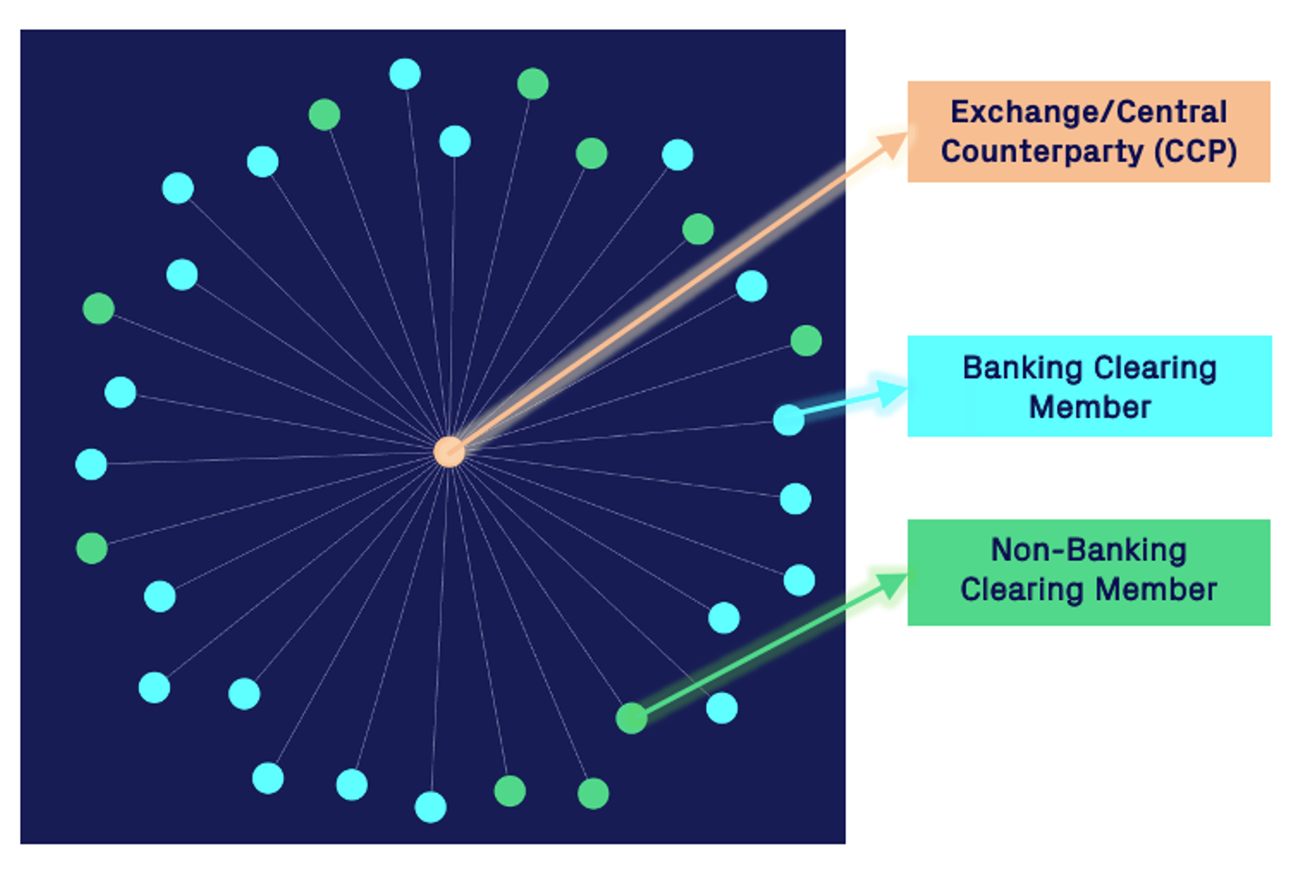
Clearing Member (Banking and non-banking):
Each Clearing Member submits buy or sell limit orders, which consist of a bid price and volume, to the CCP/Exchange.
There are two different types of CM:
- Banking CM's: which trades the asset based on its estimate of the fundamental asset value and are subject to the Basel-III minimum capital ratios; and
- Non-Banking CM's:, which are zero intelligence/noise traders that submit buy and sell limit orders at random.
We currently assume that all CM’s takes an unhedged position to minimise model complexity. The potential for each CMi to engage in hedging could be added in future versions. The cash balances Cit and total marked-to-market value of contracts (A(i,t)MTM) from each CMi are also recorded. Each CMi also contributes to a default fund based on their total exposure to the market. The default fund will be used to cover the losses in an event of a default.
Exchange (CCP):
The Exchange/CCP is responsible for maintaining the limit order book and executing the trades submitted by each CM. It also monitors the initial and maintenance margin that is required by each CM and enforces margin calls.
The CCP also has its own cash balance and contributes to a small proportion of the default fund. Default waterfall: Under the scenario where a CMi is unable to meet a margin call, the sequence of event is followed until the losses are recuperated. The severity of an event increases as the default waterfall (outlined in the next subsection) progresses downwards.
Model Steps and Details
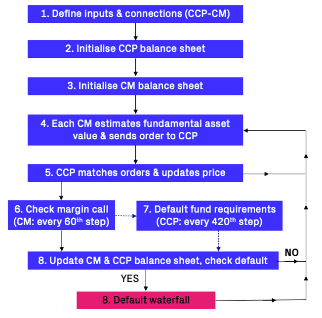
The figure below outlines the sequence of events that occurs in each time step (t), and is further elaborated:
Define Inputs and Connections (CCP & CM)
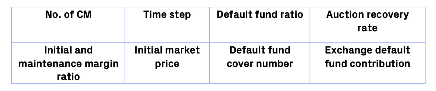
The following input parameters (table below) are required by the ABM, which can be modified to achieve the user’s goal:
Initialise CCP (Exchange) Balance Sheet
The CCP cash balance is initialised to fall within a uniform distribution of between 5,000 and 10,000. This cash balance is expected to change according to its contribution to the default fund.
Initialise CM Balance Sheet
An example of the balance sheet for each CMi is recorded in an array as shown below,
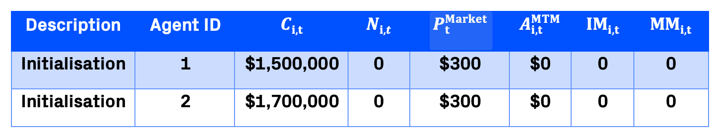
The initial cash balance of banking CM’s C(i,t_0)Bank is assumed to be uniformly distributed between 50,000,000 and 100,000,000, while the initial cash balance for non-banking CM’s C(i,t0)Non-Bank are smaller, uniformly distributed between 50,000 and 100,000. For both CM type, the initial number of open contracts N(i,t0) is set to zero. PtMarket is the market price of the instrument at time step t. A(i,t)MTM is the notional marked-to-market value of the contracts held by each CM and is calculated as shown below:

IM(i,t) and MM(i,t) are the initial margin and maintenance margin required by each CMi at a given time step,

where αIM and αMM are the initial and maintenance margin ratio, and P(i,t)Filled is the average price of which the order is filled.
Fundamental Asset Value Estimates & Order Submission
Each CMi decides whether to buy or sell the based on their estimate of the fundamental value of the asset (V(i,t)).
Banking CM’s derive an estimate of the fundamental asset value by calibrating a Brownian Bridge with daily candlestick data. In each time step, the banking CM has three options: (i) submit a buy order of volume N(i,t)Bid units if V(i,t) > P(i,t-1)Market + ∆ threshold; (ii) submit a sell order of N(i,t)Ask if V(i,t) < P(i,t-1)Market - ∆ threshold; and (iii) do nothing if the two conditions are not met.
The ∆ threshold ~ U [0.01V(i,t), 0.10V(i,t)] is set to ensure that the CM do not change their order direction when V(i,t) is very close to P(i,t-1)Market.
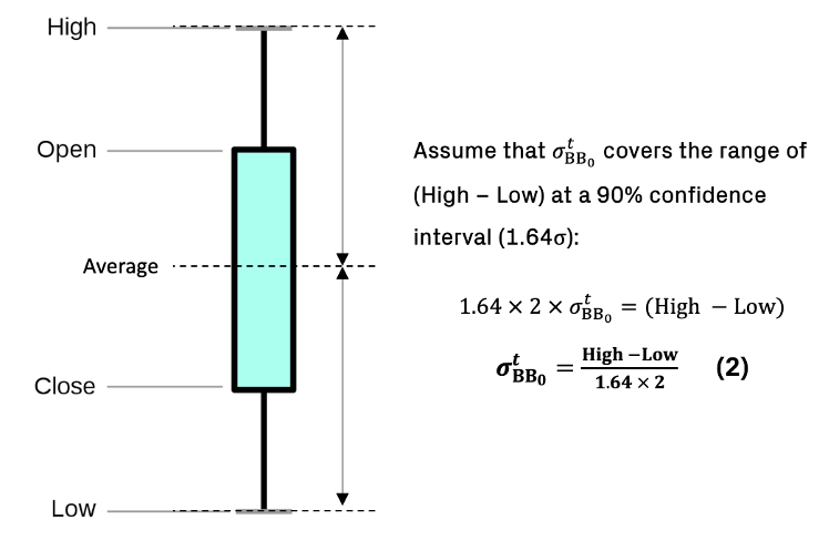
To estimate V(i,t), we used daily price data for the UK FTSE100 and FTSE250 index for two specific time periods: (i) calmer market conditions (2018 to 2019); and (ii) a stressed market environment (2008 to 2009). Each data point consists of the daily open, close, highs and lows, and a numerical method is subsequently used to estimate the daily volatility of the Brownian Bridge (σBBt) with the following steps:
Initial Guess of σ(BB0)^t
Estimate time period (thigh and tlow)
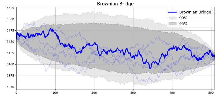
In a symmetrical Brownian Bridge where B0 = Bt, the high/low of the Brownian Bridge is expected to be at t = T/2. This is because the variance for B(t), Var[B(t)] = (t(T-t)) / T, is largest at t = T/2. However, the above property is no longer valid when B0 ≠ Bt (shown in the figure below).
The Limited-memory BFGS (L-BFGS) optimization algorithm is used to estimate tlow & thigh:
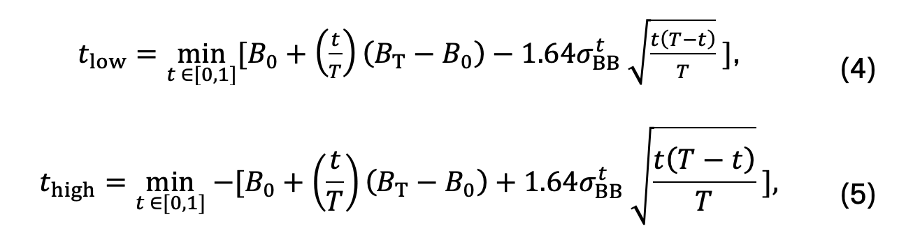
where the objective functions in Eq. (4) and Eq. (5) are the expected values of B(t) for a given σBBt at a 90% confidence interval.
Optimise σ_BB^t
The L-BFGS optimization algorithm is used to optimise σ_BB^t that satisfies the following objective function,

where the initial guess for is calculated in Eq. (3), while Blow = B(tlow) and Bhigh = B(thigh) were calculated using Eq. (4) and Eq. (5) respectively.
Essentially, the objective function in Eq. (6) minimizes the sum of squared errors for the highs and lows between the Brownian Bridge estimates and the real data. An example of V(i,t) for a given day is illustrated in the example below.
For non-banking CM’s, they have a probability of α in submitting limit orders at price P(i,t)Limit, and a probability of μ in submitting market orders. When an order is submitted by the non-banking CM, there is a probability of 0.5 of submitting either a buy or sell order. For limit orders, the price is defined as:

where Ptmid is the mid-price (between the bid-ask spread) of an asset at the end of the previous step and δp~exp(λ) is such that limit orders are placed at an exponentially distributed depth in the limit order book. Further information is available and could be made available upon request.
Order Matching & Price Updates
All orders with bid prices that are larger than the ask prices are immediately filled. An order submitted by the CM can be partially filled when there is insufficient liquidity. Any partially filled or unfilled order will remain in the CCP’s order book for the next 10 to 100-time steps, determined via a random uniform distribution. In an event where a CM submits another order with an existing order remains in the CCP’s order book, the most recent order will replace the existing order.
At the end of each time step, the CCP sends the latest instrument price and transaction reports to every CM.
Check Margin Call & Cash Rebates
Margin calls are checked by each CM at every hour (or every 60th time step). The profit/loss, (P/L)(i,t), for each CM are first calculated as follows,

A margin call is triggered if (P/L)(i,t) is negative and exceeds the maintenance margin (MM(i,t)). The required cash to restore the initial margin (IM(i,t)) will be deducted from the cash balance of the affected CM (C(i,t)). Conversely, any excess profits, (P/L)(i,t) > 0, will be credited to C(i,t):
if abs((P/L)(i,t)) > MM(i,t),

Once this is complete, every CM will send the updated balance sheet to the CCP. The conditions for a default will be checked as highlighted in Section 3.8.
Default Fund Requirements and Allocation
The default fund requirements are recalculated at every 420th time step, representing one trading day (7 hours). The size of the default fund that is required from the CCP is determined using the COVER II rule: the default fund has to be able to cover the default of the CM with the largest exposure, or of the second and third largest CM if the summation of their exposure is greater than the largest CM4.
These CM’s are subjected to extreme yet plausible market scenarios, and for this reason, we specify a 30% change in the underlying instrument value to simulate the potential losses that could be incurred by each CM,

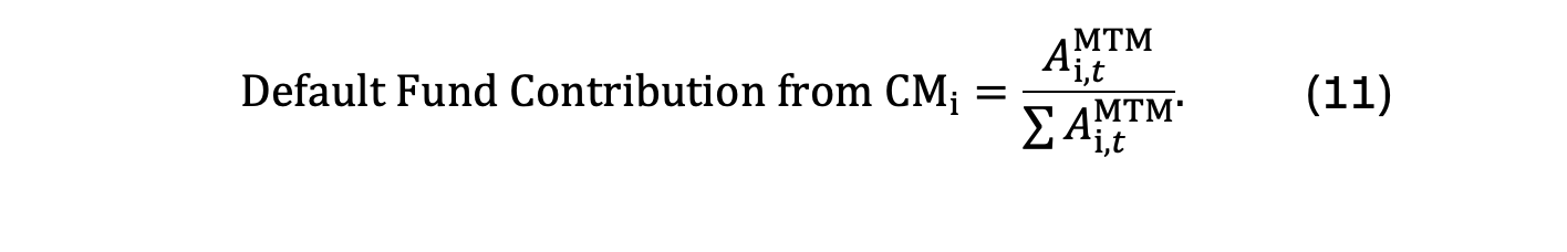
Once this is complete, the default fund size will be equal to: (i) the largest value of Lossi; or (ii) the summation of second and largest value of Lossi if it is greater than (i). The CCP will allocate a proportion of its cash for 10% of the required default fund size, while the remaining 90% is allocated to each CM according to their respective exposure,
Check for Defaults
A default occurs when one or multiple CM’s faces a margin call and its C(i,t) is insufficient to cover the variation margin. To recover the losses of the defaulted CM, the default waterfall procedure (outlined below) is performed:
- LEVEL 1: Defaulted CM’s remaining initial margin and default fund contribution.
- LEVEL 2: CCP’s own contribution to the default fund.
- LEVEL 3: Surviving CM’s default fund contribution.
- LEVEL 4: Call for rights-of-assessment, where surviving CM’s cash balances are reduced (equal to their initial default fund contribution).
- LEVEL 5: Contribution from CCP’s own cash balances.
The severity of the default (Levels 1-5) is recorded for post analysis. For defaults that falls within Levels 1 to 4, the defaulted CM is removed from the simulation. The simulation ends if severity of default reaches Level 5.
References
- Cesa, M. (2020) Small, speculative clearing members – are they worth the risk? Risk Publications – January 2020.
- Bodie, Z., Kane, A. and Marcus, A.J., 2015. Portfolio management. McGraw Hill/Learning Solutions.
- https://www.cmegroup.com/trading/energy/crude-oil/light-sweet-crudecontractspecifications.html
- Capponi, A., Wang, J. & Zhang, H. (2018) Designing Clearinghouse Default Funds.
- Vytelingum, P. & Goremykina, A (2020) A Zero-Intelligence Agent-based Market Simulator