Financial Vulnerability Model
Last updated on 21st April 2026
Introduction
The docs and implementation overview below are based on the publicly available paper: An Agent-Based Model for Financial Vulnerability
The model, as presented in the original paper, considers assets which change in value via a random walk but can also be negatively affected by event-driven sales from hedge funds or trading desks within banks. On each time-step, hedge funds and trading desks calculate their assets under management and adjust their strategy depending on leverage limits specified in the model.
After deciding their strategy (e.g., level of buy/sell for each asset) they request funding from their relevant avenues to support their leveraged investments. Exogenous shocks on asset prices or haircuts within the model can result in over-leveraged trading entities or into a shortage of funding, which can both lead to event-driven sales and negative feedback loops within the financial system. These cascading failures that occur due to the network nature of the model, can lead to significant crises and even defaults within the model.
Recent developments, like the Archegos Capital Management crisis, or the increasing awareness of financial institutions to climate change and its effects on the financial system, are driving the adoption of computational models for scenario analysis and policy design. Variants of the FVM can explore the viability of new or existing policies, and in general, the resilience of financial systems to exogenous or endogenous shocks of any underlying cause (e.g., climate change).
Implementation Overview and Results
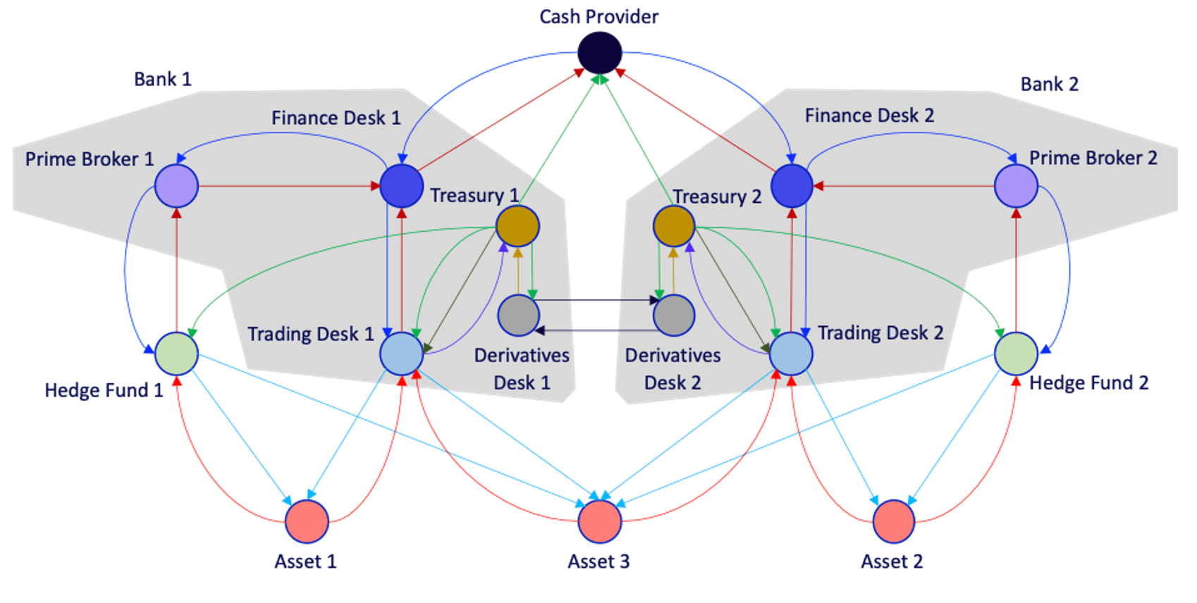
The model can be initialized by specifying the connectivity and agent parameters within a parameters json file. As such, the new SDK implementation is not bound to the 1-2-2-3 scenario, but any type of network could be specified. The Simudyne Framework reads the parameters file and creates the agents and their connectivity accordingly.
More specifically, due to the distributed execution of the Simudyne ABM framework, we built the agent network with the use of a NetworkHandler agent, which reads the parameter links and creates a HashMap of the agent positions as keys and agent IDs as values. The NetworkHandler then instructs the creation of links between FVM agents by accessing their ID from the HashMap mentioned above.
To improve the quality of the code, in terms of scalability, compactness, and readability, we implemented good coding practices such as informative naming of methods, variables and classes, base / abstract classes, and inheritance. In terms of core features, which were missing from the initial SDK implementation, the new codebase now includes updating of the haircut and creditworthiness of banks.
Furthermore, we also included a class which ensures asset correlation if pair-wise asset correlations are specified by the user. The user specifies the correlations between different assets, and the model formulates a valid correlation matrix using Eigen Decomposition to adjust any negative (invalid) Eigen values. We then use Cholesky Decomposition to obtain correlated random variables which are then sent to the assets as inputs.
Below we can see asset price variation for different assets after a 15% price shock on asset 0 at the 20th time step.
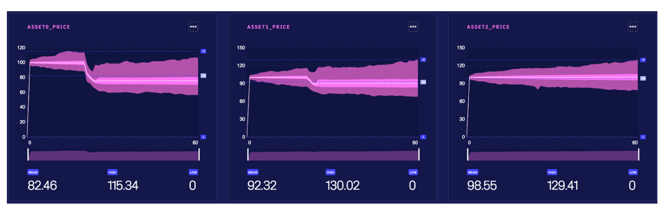
Similar contagion effects were also observed between trading entities such as hedge funds and trading desks. It is worth noting that such effects on assets are present after asset shocks, even if there is no observed correlation between the assets before the shock.
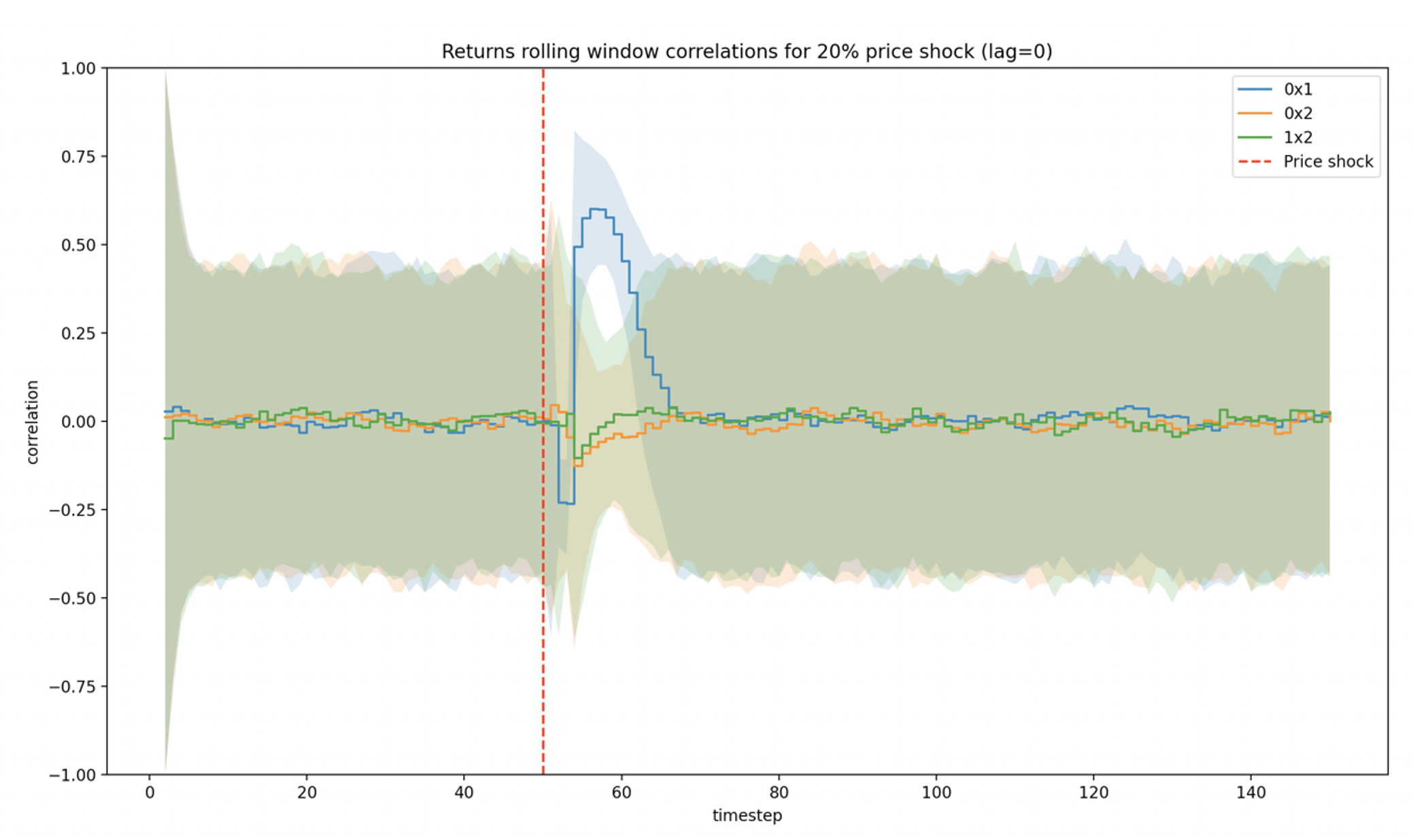
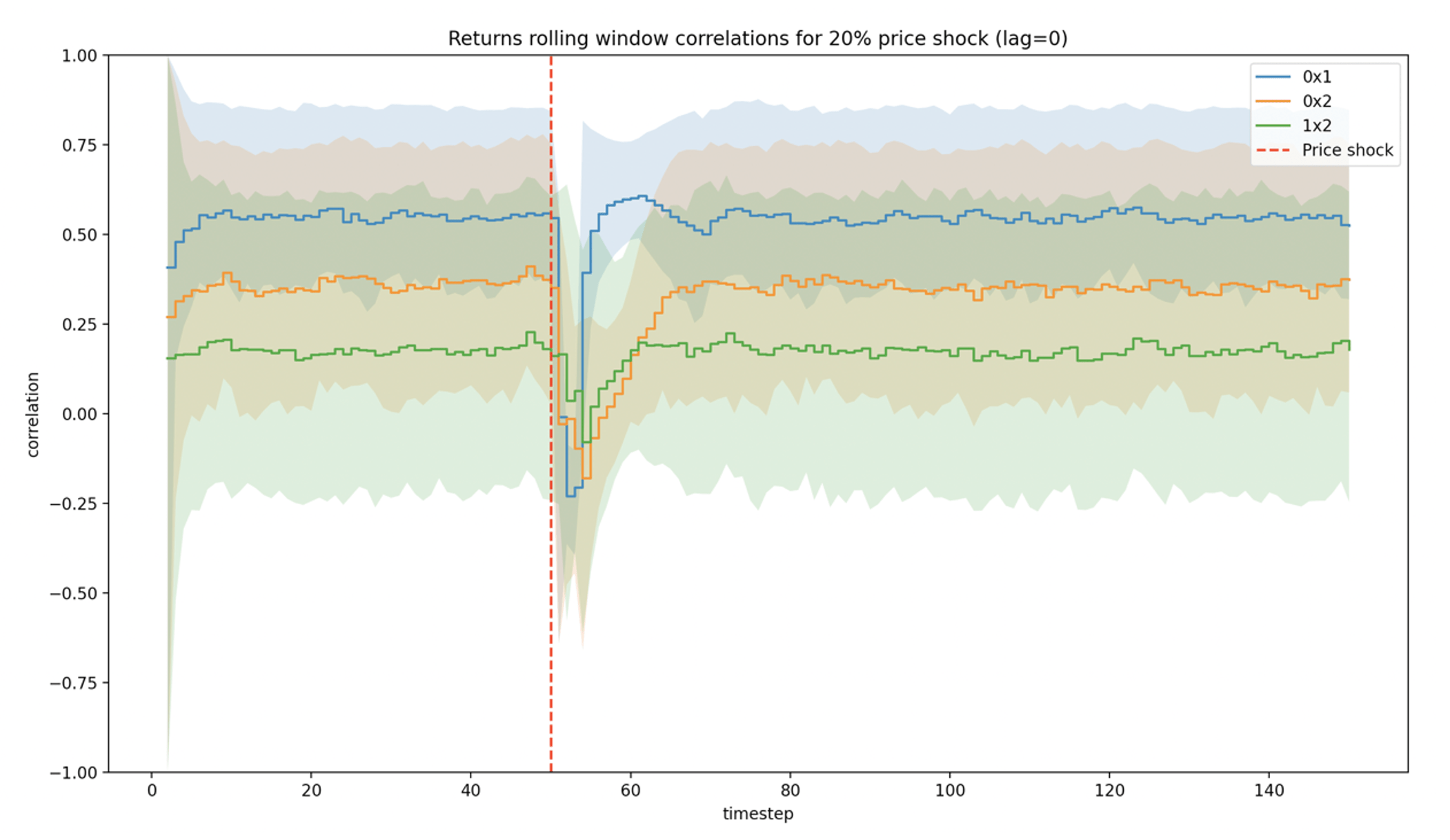
To further analyze this effect, we examined the correlation regime between assets before and after a price shock. Specifically, we were able to produce a change in correlation structure because of the architecture of the ABM and the feedback loops that result after the shock. Figure 4 and Figure 5 outline the change in regime after a 20% price shock on the 50th time step for a test of the 1-2-2-3 scenario with 1000 runs.
Below we see a change in correlation regime between initially uncorrelated asset pairs for a 20% price shock on asset 0:
Additionally, here we see change in correlation regime between initially correlated asset pairs for a 20% price shock on asset 0.:
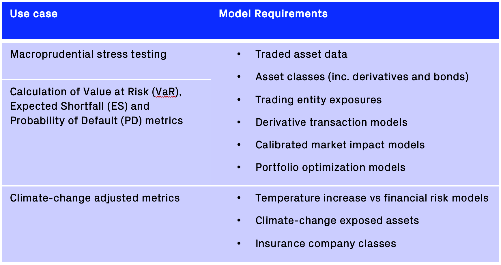
Model Extensions and Use Cases
Potential applications and use cases of the model are presented below: