Section 5: Worked Examples

This section presents four detailed model walkthroughs that showcase different facets of the SDK. Each includes source code, configuration, mechanism descriptions, simulation output, and results interpretation. The models are chosen to demonstrate spatial contagion on a grid, network-based systemic risk, competitive market dynamics with adaptive learning, and continuous-space swarm intelligence with pheromone fields.

The SDK ships with 24 complete models across 10 domains and 30 runnable example scripts covering ~95% of the API surface. Examples are organised into themed subdirectories: basics/, testing/, evaluation/, visualization/, agents/, infrastructure/, backends/, analytical/, and topologies/. See Appendix D for the full model catalog and examples/models/README.md for the complete index with SDK feature tags.

Plot rule: When Monte Carlo ensemble plots exist (median + percentile envelope), do NOT include single-seed time series plots — the MC plot subsumes them. Single-seed plots are only shown for models without MC evaluation (e.g., ant_colony spatial snapshots).

Featured model: The Global Supply Chain (supply_chain_v3) demonstrates Space2D with geographic coordinates, GeoMap visualisation in the frontend (Leaflet + CartoDB with tiered hub routing and antimeridian splitting), 5 named scenarios, and 100-seed Monte Carlo evaluation. It is the most complete example of the SDK's continuous-space and geospatial capabilities.

5.1 Forest Fire --- Spatial Contagion on a Grid

Overview

The forest fire model is the simplest spatial model in the SDK library. Cell agents on a 2D grid transition through three irreversible states: TREE, BURNING, and ASH. Fire spreads from burning cells to adjacent tree cells via Von Neumann (4-connected) neighbourhood messaging. Spontaneous ignition models lightning strikes. The model exhibits percolation dynamics: below a critical tree density, fire cannot spread far; above it, the fire front propagates as a connected wavefront that consumes most of the forest.

This model demonstrates: GridSpace, spatial neighbourhood messaging via broadcast(), cell-based state transitions, GlobalState for shared parameters, and the standard accumulator pattern.

Mechanisms

Mechanism	Hypothesis	Parameters
Fire spread	Fire propagates through spatial adjacency. Burning cells ignite neighbouring tree cells, producing percolation-like wavefront dynamics.	tree_density
Spontaneous ignition	Random ignition events (lightning) model exogenous fire starts independent of existing fires.	ignition_prob

Agent and Message Types

A single agent type (Cell) with state {cell_state: str, row: int, col: int} and one message type (FireSpread, a signal-only Message subclass). The model uses two phases in a Sequence: burning cells broadcast FireSpread in Phase 1, and all cells process messages and update state in Phase 2.

Source Code

from simudyne.engine.sdk import ABMModel, Agent, Action, GlobalState, Message, Sequence
from simudyne.engine.space import GridSpace

class FireSpread(Message):
    """Notification that an adjacent cell is on fire."""
    pass

class Cell(Agent):
    __state_schema__ = {"cell_state": str, "row": int, "col": int}

    def __init__(self, agent_id, model=None):
        super().__init__(agent_id=agent_id, model=model)
        self.cell_state = "EMPTY"
        self.row = 0
        self.col = 0

def _spread_fire(cell):
    """Phase 1: Burning cells notify neighbours."""
    if cell.cell_state == "BURNING":
        cell.broadcast(FireSpread, link_type="grid")

def _update_state(cell):
    """Phase 2: Process fire messages and transition state."""
    if cell.cell_state == "BURNING":
        cell.cell_state = "ASH"
        cell.get_accumulator("ash").add(1)
        return
    if cell.cell_state == "TREE":
        if cell.get_messages(FireSpread):
            cell.cell_state = "BURNING"
            cell.get_accumulator("burning").add(1)
            return
        if cell.rng.random() < cell.get_globals().ignition_prob:
            cell.cell_state = "BURNING"
            cell.get_accumulator("burning").add(1)
            return
        cell.get_accumulator("trees").add(1)
    elif cell.cell_state == "ASH":
        cell.get_accumulator("ash").add(1)

class ForestFireModel(ABMModel):
    def init(self):
        self.register_agent_type("Cell", Cell)
        self.register_link_type("grid", "Cell", "Cell")
        for name in ("trees", "burning", "ash"):
            self.create_accumulator(name)

    def setup(self, config):
        super().setup(config)
        rows = config.get("grid_rows", 30)
        cols = config.get("grid_cols", 30)
        density = config.get("tree_density", 0.6)
        self.set_globals(GlobalState(ignition_prob=config.get("ignition_prob", 0.001)))

        cells = self.create_agents("Cell", rows * cols)
        grid = GridSpace(self, rows=rows, cols=cols, wrap=False, link_type="grid")

        import numpy as np
        init_rng = np.random.default_rng(self._seed + 100)
        for i, agent in enumerate(cells):
            r, c = i // cols, i % cols
            agent.row, agent.col = r, c
            grid.place_agent(agent, (r, c))
            agent.cell_state = "TREE" if init_rng.random() < density else "EMPTY"

        # Ignite centre cell
        for a in grid.get_agents_at((rows // 2, cols // 2)):
            if a.cell_state == "TREE":
                a.cell_state = "BURNING"

    def step(self):
        self.reset_accumulators()
        self.run(Sequence(
            Action.create(Cell, _spread_fire),
            Action.create(Cell, _update_state),
        ))
        self.record_accumulators()

Configuration

{"seed": 42, "steps": 100, "grid_rows": 30, "grid_cols": 30,
 "tree_density": 0.6, "ignition_prob": 0.001}

Running and Results

model = ForestFireModel.run_simulation({
    "seed": 42, "steps": 100, "grid_rows": 30, "grid_cols": 30,
    "tree_density": 0.6, "ignition_prob": 0.001,
})

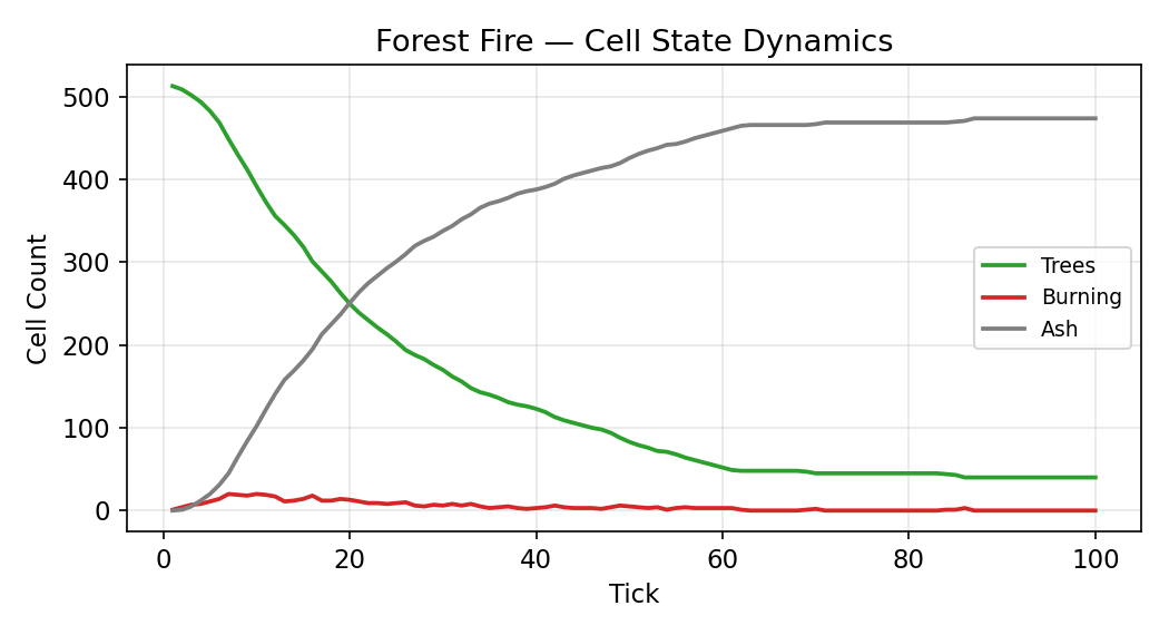
At tree_density=0.6 (near the percolation threshold for a 4-connected grid ~0.59), the fire spreads as a roughly circular wavefront from the centre, consuming connected tree clusters while stopping at gaps in the canopy. The plot shows the characteristic dynamics: trees (green) decreases monotonically as the fire front advances, burning (red) peaks in the early ticks as the wavefront reaches maximum width, then decays as fuel is exhausted, and ash (grey) accumulates to a final value of ~475 cells — the connected cluster reachable from the ignition point. The remaining ~40 trees are in disconnected patches that the fire cannot reach.

---

5.2 Gai-Kapadia --- Systemic Risk Contagion

Overview

The Gai-Kapadia model simulates interbank contagion on a scale-free network. Banks hold interbank exposures and cash buffers. When a bank defaults, the losses propagate through the network: if the fraction of defaulted neighbours weighted by exposure exceeds a bank's cash buffer, that bank also defaults. The model is a faithful port of the Simudyne Java SDK reference implementation.

This model demonstrates: NetworkSpace with scale_free topology, heterogeneous agent initialisation, threshold-based contagion mechanics, the Sequence phase ordering guarantee, and GlobalState for shared parameters.

Mechanisms

Mechanism	Hypothesis	Parameters
Threshold contagion	Bank defaults propagate through interbank exposures. When defaulted_fraction * interbank_exposure > cash_buffer, the bank defaults.	cash_buffer, interbank_pct
Scale-free topology	Barabasi-Albert preferential attachment concentrates systemic risk at highly-connected hub banks, producing realistic fragility where a single hub failure cascades.	num_banks, network_m
Heterogeneous buffers	Uniform variation in cash buffers (buffer_heterogeneity) produces realistic partial cascades: well-capitalised banks survive while weaker banks fail.	buffer_heterogeneity

Agent and Message Types

One agent type (Bank) with state {status: str, cash_buffer: float, interbank_exposure: float} and one message type (DefaultNotification, signal-only). Two phases: defaulted banks broadcast notifications (Phase 1), then solvent banks check if losses exceed their buffer (Phase 2). The phase ordering guarantees that every bank sees all neighbour defaults before making its solvency decision.

Source Code

from simudyne.engine.sdk import ABMModel, Agent, Action, GlobalState, Message, Sequence
from simudyne.engine.topology import scale_free

class DefaultNotification(Message):
    pass

class Bank(Agent):
    __state_schema__ = {"status": str, "cash_buffer": float, "interbank_exposure": float}

    def __init__(self, agent_id, model=None):
        super().__init__(agent_id=agent_id, model=model)
        self.status = "SOLVENT"
        self.cash_buffer = 0.04
        self.interbank_exposure = 0.2

def _send_state(bank):
    if bank.status == "DEFAULT":
        bank.broadcast(DefaultNotification, link_type="interbank")

def _update_balance_sheet(bank):
    if bank.status != "SOLVENT":
        bank.get_accumulator("total_defaults").add(1)
        return
    messages = bank.get_messages(DefaultNotification)
    num_neighbors = len(bank.get_links("interbank"))
    if num_neighbors > 0 and len(messages) > 0:
        loss = (len(messages) / num_neighbors) * bank.interbank_exposure
        if loss > bank.cash_buffer:
            bank.status = "DEFAULT"
            bank.get_accumulator("total_defaults").add(1)
            return
    bank.get_accumulator("solvent_count").add(1)

class GaiKapadiaModel(ABMModel):
    def init(self):
        self.register_agent_type("Bank", Bank)
        self.register_link_type("interbank", "Bank", "Bank")
        self.create_accumulator("total_defaults")
        self.create_accumulator("solvent_count")

    def setup(self, config):
        super().setup(config)
        n = config.get("num_banks", 100)
        buf = config.get("cash_buffer", 0.06)
        het = config.get("buffer_heterogeneity", 0.95)

        self.set_globals(GlobalState(num_banks=n, cash_buffer=buf,
                                     interbank_pct=config.get("interbank_pct", 0.2)))
        banks = self.create_agents("Bank", n)

        import numpy as np
        rng = np.random.default_rng(self._seed + 200)
        for b in banks:
            if het > 0:
                b.cash_buffer = float(rng.uniform(buf * (1 - het), buf * (1 + het)))
            else:
                b.cash_buffer = buf
            b.interbank_exposure = config.get("interbank_pct", 0.2)

        scale_free(self, "Bank", "interbank", m=config.get("network_m", 2))
        banks[config.get("shock_bank_id", 0)].status = "DEFAULT"

    def step(self):
        self.reset_accumulators()
        self.run(Sequence(
            Action.create(Bank, _send_state),
            Action.create(Bank, _update_balance_sheet),
        ))
        self.record_accumulators()

Configuration

{"seed": 184, "steps": 100, "num_banks": 100, "cash_buffer": 0.06,
 "interbank_pct": 0.2, "shock_bank_id": 0, "buffer_heterogeneity": 0.95}

Running and Results

model = GaiKapadiaModel.run_simulation({
    "seed": 184, "steps": 100, "num_banks": 100,
    "cash_buffer": 0.06, "interbank_pct": 0.2,
    "shock_bank_id": 0, "buffer_heterogeneity": 0.95,
})

The contagion unfolds in waves: the initial default triggers notifications to the shocked bank's neighbours (step 1), those with insufficient buffers default and propagate further (step 2-5), and the cascade either dies out (if buffers are sufficient) or reaches a significant fraction of the network. The plot shows the cascade dynamics: defaults (red) rise rapidly over the first ~15 ticks as the contagion propagates through weakly-capitalised banks, then stabilise at 50 defaults as the remaining solvent banks (blue) have sufficient buffers to absorb the losses. With buffer_heterogeneity=0.95, banks have buffers ranging from near-zero to ~0.12, producing realistic partial cascades where well-capitalised banks act as firewalls. The total_defaults accumulator tracks cascade depth, and solvent_count tracks the surviving banking system. The model exhibits a sharp phase transition in cash_buffer: small reductions cause disproportionately larger cascades.

---

5.3 Credit Card Competition --- Adaptive Market Dynamics

Overview

The credit card model is the most complex example in the library: a two-sided market where 200 heterogeneous households choose between two credit card providers (Phoenix Bank and Villagebank) based on interest rates and reward programmes. Providers adaptively adjust their rates using a Delta Learning (Widrow-Hoff) rule to compete for market share. The model is a faithful port of the Simudyne Java SDK credit card model (v2.6.0-RC4).

This model demonstrates: bipartite link topologies (providers ↔ households), multiple message types with typed payloads, the Sequence/Action ordering for multi-phase market interactions, adaptive agent learning, empirical income distributions, and the Bank of England consumption model.

Mechanisms

Mechanism	Hypothesis	Parameters
Adaptive rate competition	Providers use Delta Learning to adjust rates: below-target market share triggers rate cuts proportional to ms/prevMs; above-target triggers increases.	ell1, ell2, freq1, freq2, msTarget1, msTarget2
Utility-based balance split	Households split spending using f_i = max(0.005, rate_i - reward_i * creditScore^2). Higher credit scores amplify reward sensitivity.	rewardWeight1, rewardWeight2, ellH, creditCardUsage
Bank of England consumption	Discretionary consumption follows minLiqWealth = 4.07 * ln(income - 5900) - 33.1 + N(0,1), creating realistic wealth dynamics.	incomeVolatility
Transactor/revolver dynamics	Households with wealth > totalBalance and creditScore > 0.8 pay full balance (transactors); others pay partial amounts (revolvers).	minPayment, avgPayment
Reward programme	Phoenix Bank's reward factor lowers effective rate for high-score households, capturing market share without reducing nominal rate.	rewardWeight1, hasRewardShock

Agent and Message Types

Two agent types: Household (200 agents with income, wealth, credit score, balances on two cards, learning rate) and CreditCardProvider (2 agents with rate, adaptive rate, learning rate, market share). Four message types: CreditCardOffer1 and CreditCardOffer2 (provider → household, carrying rate and reward factor) and Balance1 and Balance2 (household → both providers, carrying balance and credit score).

The link topology is bipartite: each provider links to all households for sending offers, and each household links to both providers for sending balance reports. This requires four link types (provider1_household, provider2_household, balance_link1, balance_link2).

Execution Phases

The model executes in four phases per step:

1. Household step (single Action): Income shock (±2.5%), earn income, subsistence consumption, pay card (transactor vs revolver logic).
2. Provider send offer (Sequence Phase 1): Each provider broadcasts rate and reward factor to all linked households.
3. Household discretionary consumption (Sequence Phase 2): Households receive offers, compute utility-based balance split, allocate spending, send balance reports to both providers.
4. Provider update offer (Sequence Phase 3): Providers estimate market share from balance messages and adapt rates using Delta Learning.

Phase ordering is critical: providers must send offers before households consume, and households must send balances before providers update rates. The Sequence guarantees this.

Configuration

{
  "seed": 42, "steps": 200, "nbConsumers": 200,
  "rateOne": 0.1, "rateTwo": 0.1,
  "rewardWeight1": 0.5, "rewardWeight2": 0.0,
  "msTarget1": 0.65, "msTarget2": 0.5,
  "ell1": 0.02, "ell2": 0.02, "ellH": 0.05,
  "creditCardUsage": 0.1, "minPayment": 0.05, "avgPayment": 0.2,
  "noise": 0.05, "incomeVolatility": 2.5,
  "freq1": 3, "freq2": 3, "hasRewardShock": false
}

Running and Results

from examples.models.credit_card.model import CreditCardModel

model = CreditCardModel.run_simulation({"seed": 42, "steps": 200})

The model produces five key dynamics:

1. Market share convergence: Phoenix Bank captures ~64% market share via its reward programme, despite identical initial rates. Villagebank stabilises at ~36%.
2. Rate divergence: Phoenix Bank raises rates from 0.10 to ~0.11 (exploiting its market position), while Villagebank reduces rates to ~0.04 to remain competitive. This is a Nash equilibrium: neither provider can improve by unilaterally changing strategy.
3. Balance accumulation: Aggregate household debt grows exponentially as revolving balances compound with interest, reflecting real-world credit card debt dynamics.
4. Risk-weighted exposure asymmetry: Phoenix Bank's RWE is lower despite higher balances because it attracts higher credit-score households (who are more reward-sensitive), while Villagebank's RWE is disproportionately high due to its lower-score customer base.
5. Transactor/revolver split: ~20-30% of households are transactors (pay in full each month), while the rest are revolvers whose partial payments cause balance growth.

Setting hasRewardShock=true removes Phoenix Bank's reward programme at step 100, causing a dramatic rebalancing: market shares converge, rates converge, and the system reaches a new symmetric equilibrium. This demonstrates the model's capacity for counterfactual analysis.

---

5.4 Ant Colony --- Stigmergic Foraging on Continuous Space

Overview

The ant colony model simulates pheromone-based foraging on a continuous 2D toroidal world. Ants navigate between a central nest and four food sources at the corners using indirect communication through pheromone trails (stigmergy). This is the only model in the library that uses no links and no messages --- all coordination emerges from agents depositing and sensing scalar fields in the environment.

This model demonstrates: Space2D (continuous coordinates with spatial hash grid), FieldLayer (pheromone deposition, sampling, evaporation, diffusion), Space2DEnvironment (push-based observations with visibility configuration), the environment-as-mediator pattern, and Weber-Fechner psychophysical gradient response.

Mechanisms

Mechanism	Hypothesis	Parameters
Pheromone stigmergy	Ants deposit pheromones that evaporate over time, creating decaying trails. Other ants follow gradients, producing emergent shortest-path behaviour without direct communication (Deneubourg et al. 1990).	evaporation_rate, diffusion_rate
Weber-Fechner gradient following	Ants bias movement toward higher pheromone concentrations using logarithmic response: weight = alpha * log(1 + beta * gradient_magnitude). Stronger trails attract more ants (positive feedback) but response saturates, preventing total lock-in.	weber_alpha, weber_beta, weber_max_weight
Random exploration	Gaussian noise on heading enables discovery of new food sources and prevents premature convergence to suboptimal trails.	noise_sigma
Two-pheromone system	Bidirectional pheromone trails — food_pheromone guides foragers toward food, home_pheromone guides returning ants toward the nest — enable efficient round-trip navigation.	(structural)
Beacon emission	Nest and food sources emit constant pheromone independent of ant traffic, providing persistent homing signals even when ant density is low.	nest_beacon_strength, food_beacon_strength

Agent and Space Types

One agent type (Ant) with state {state: str, speed: float, direction: float, found_at_tick: int, cumulative_distance: float}. No message types — ants communicate exclusively through the pheromone field layers. The environment (Space2DEnvironment) pushes observations containing pheromone gradients to each ant only when its vicinity has changed (dirty-cell tracking).

Three phases in a Sequence: ants sense gradients and move (Phase 1), ants interact with food sources and the nest (Phase 2), and ants deposit pheromone at their current position (Phase 3). After the agent phases, the model applies evaporation and diffusion to both pheromone layers and emits beacon signals at the nest and food source locations.

Source Code (Key Excerpts)

from simudyne.engine.sdk import ABMModel, Agent, Action, Sequence
from simudyne.engine.space2d import (
    FieldLayer, Space2D, Space2DEnvironment, VisibilityConfig, VisibilityLevel,
)

class Ant(Agent):
    __state_schema__ = {"state": str, "speed": float, "direction": float,
                        "found_at_tick": int, "cumulative_distance": float}

def _sense_and_move(ant):
    """Follow pheromone gradient with Weber-Fechner response + noise."""
    obs = model.env.observe(ant)
    grad = obs["layer_gradients"].get(
        "food_pheromone" if ant.state == "FORAGING" else "home_pheromone", (0, 0))
    grad_mag = math.sqrt(grad[0]**2 + grad[1]**2)
    if grad_mag > 1e-6:
        weight = min(alpha * math.log(1 + beta * grad_mag), max_weight)
        ant.direction = (1 - weight) * (ant.direction + noise) + weight * math.atan2(*grad[::-1])
    model.env.move_agent(ant, x + speed * math.cos(ant.direction),
                                y + speed * math.sin(ant.direction))

def _interact(ant):
    """Pick up food at sources, deposit at nest."""
    if ant.state == "FORAGING" and near_food:
        ant.state = "RETURNING"; ant.direction += math.pi
    elif ant.state == "RETURNING" and near_nest:
        ant.state = "FORAGING"; ant.get_accumulator("food_collected").add(1)

def _deposit_pheromone(ant):
    """Deposit trail pheromone: food_pheromone when returning, home_pheromone when foraging."""
    if ant.state == "FORAGING":
        model.home_layer.deposit(x, y, 1.0)
    else:
        model.food_layer.deposit(x, y, 1.0)

class AntColonyModel(ABMModel):
    def setup(self, config):
        super().setup(config)
        self.env = Space2DEnvironment(width=50, height=50, wrap=True, cell_size=5,
            visibility=VisibilityConfig(level=VisibilityLevel.ANONYMOUS, default_radius=5))
        self.env.attach(self)
        self.food_layer = self.env.space.add_layer("food_pheromone", 100, 100)
        self.home_layer = self.env.space.add_layer("home_pheromone", 100, 100)
        # Place 2000 ants at nest (centre), 4 food sources at corners

    def step(self):
        self.reset_accumulators()
        self.env.step()  # Push observations to agents with dirty vicinities
        self.run(Sequence(
            Action.create(Ant, _sense_and_move),
            Action.create(Ant, _interact),
            Action.create(Ant, _deposit_pheromone),
        ))
        # Beacon emissions at nest and food sources
        self.home_layer.deposit(cx, cy, nest_beacon_strength)
        for fx, fy, _ in self.food_sources:
            self.food_layer.deposit(fx, fy, food_beacon_strength)
        # Environment dynamics
        self.food_layer.evaporate(0.01); self.home_layer.evaporate(0.01)
        self.food_layer.diffuse(0.03);   self.home_layer.diffuse(0.03)

Configuration

{"seed": 42, "steps": 200, "n_ants": 2000, "world_size": 50.0,
 "ant_speed": 2.0, "evaporation_rate": 0.01, "diffusion_rate": 0.03,
 "layer_resolution": 100, "nest_radius": 5.0, "food_radius": 5.0,
 "visibility_radius": 5.0, "nest_beacon_strength": 200.0,
 "food_beacon_strength": 100.0, "weber_alpha": 0.3, "weber_beta": 100.0,
 "weber_max_weight": 0.8, "noise_sigma": 0.4}

Running and Results

from examples.models.ant_colony.model import AntColonyModel, model_config

model = AntColonyModel.run_simulation(model_config)

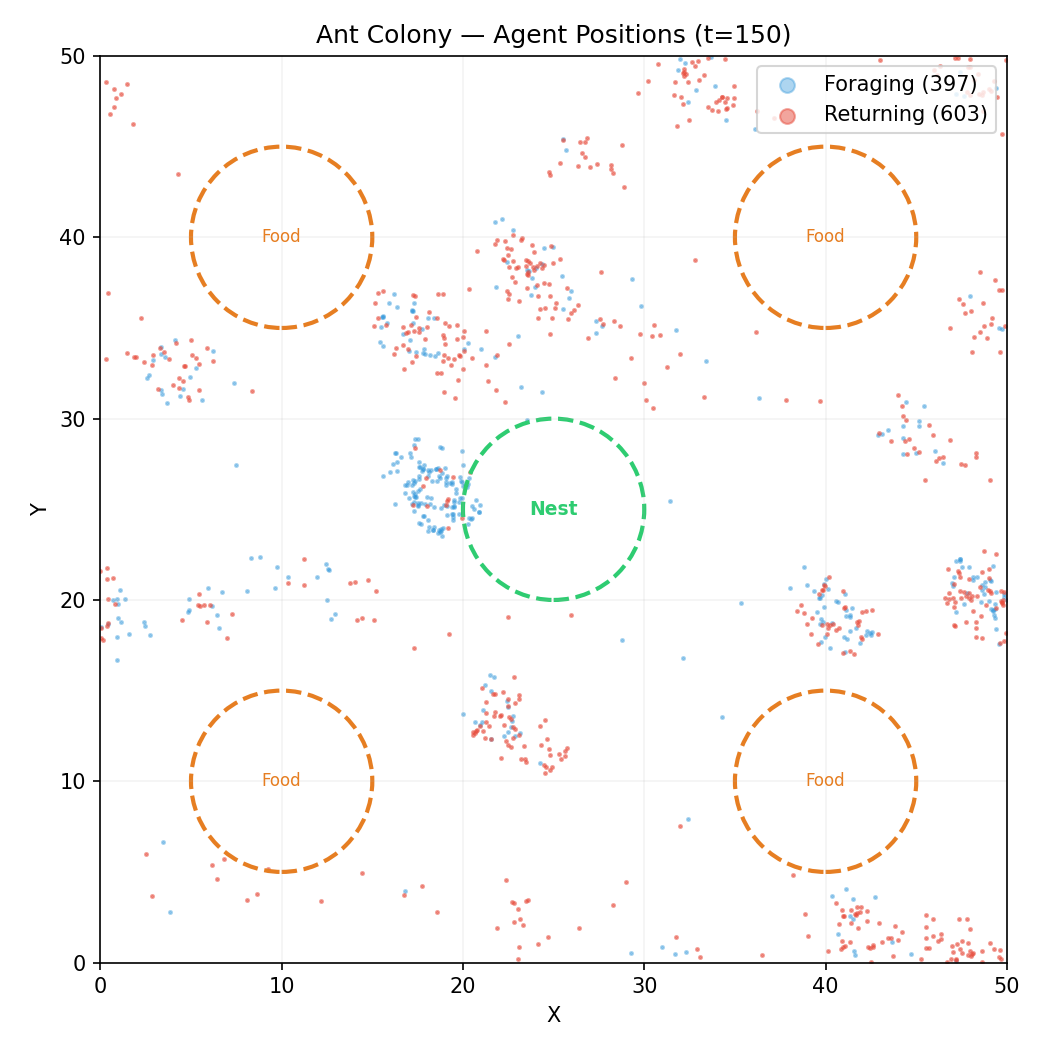
The positions plot shows the spatial distribution of 1,000 ants at tick 150. Blue dots are foraging ants (searching for food), red dots are returning ants (carrying food back to the nest). The central green circle marks the nest, and the four orange circles mark food sources at the corners. Ants cluster along emergent trails between the nest and food sources — these trails are not hard-coded but arise from pheromone-mediated positive feedback.

The pheromone field heatmaps (log scale) reveal the information structure underlying the trails. The food pheromone (left, warm colours) is deposited by returning ants and guides foragers toward food sources — note the four hot spots at food locations and the diffuse trails connecting them to the centre. The home pheromone (right, cool colours) is deposited by foraging ants and guides returning ants back to the nest — note the strong concentration at the nest (centre) radiating outward. The log scale reveals that pheromone concentration spans three orders of magnitude, with beacon emissions creating persistent local maxima that anchor the trail network.

The time series plots show foraging performance and pheromone dynamics. The left panel shows foraging performance: food_found (green) spikes in the early ticks as the initial burst of ants reaches the four food sources, then settles into a sustained but variable collection rate as pheromone trails form and stabilise. food_collected (orange) follows with a delay equal to the round-trip time. The right panel shows pheromone dynamics: both food_pheromone (red) and home_pheromone (blue) grow as trails are reinforced, with food pheromone growing faster due to the higher beacon strength at food sources. The system approaches a dynamic steady state where deposition balances evaporation.

The model tracks four Stage C metrics: mean_round_trip_time (average ticks for a food-nest round trip — measures trail efficiency), trail_efficiency_ratio (actual path length / straight-line distance — measures path optimality), pheromone_gini (Gini coefficient of pheromone distribution — measures trail concentration), and exploration_coverage (fraction of grid cells visited — measures spatial coverage). An ablation study (single_pheromone=True) disables the two-pheromone system, demonstrating that bidirectional signalling significantly reduces round-trip time compared to a single-pheromone baseline.