What is System Dynamics?

System Dynamics is an approach to understand complex nonlinear systems via the creation of stocks, flows, delays, and feedback loops. Originally developed in the 1950's to model industrial or factory processes it has shown usage in understanding and mapping large complex systems to enact policies in the fields of trade, banking, regulation, and more.

In relation to Agent-Based Modelling, System Dynamics can be better thought of as the 'top-down' approach to modelling a complex system instead of bottom up. However, there have been some interesting studies about the combination of these two approaches such as Combining system dynamics and agent-based modelling to analyze social-ecological interactions, Martin, R., M. Schlüter 2015

Stocks and Flows

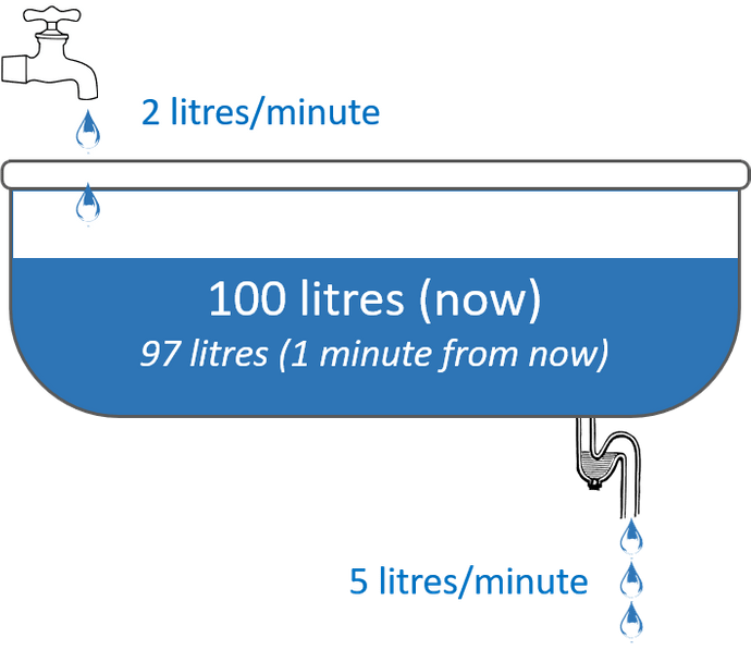
A good metaphor for a stock is to think of it as a bathtub. There is a level of water in the bathtub, and there are two pipes that allow water to flow in and out of the tub.

A flow is thought of as the amount of water that physically moves through the pipes. This change in the value dependent on whether it's leaving or entering the tub (stock) will alter the value of a connected stock.

The below image gives an example of what this can look like in a very basic case with 1 stock and 2 flows. Note that we've not replicated the entire ecosystem of water here despite that being something one could easily do with System Dynamics modelling. As you'll see building these types of models there's room for simplifications such as having the water come from a known 'source'.

Stock & Flow modelling then is the process of breaking down a complex system into testable, and interrogatable sections of resources, and how those resources are moved by flows.

The goal is to analyze to see where the breakpoints or bottlenecks exist, identify which variables alter or improve the overall outcome, and what feedback loops exist and how this affects the model as a whole.

Variables & Delays

When building a System Dynamics model there will be two other components you'll want to use. The first is the variables. These are values or functions that resolve to a number to be used most commonly by other variables or flows.

These variables do not directly alter the 'course' of the model by which we mean stocks&flows. Variables instead indirectly change the value of a flows rate thus altering the entire system.

A Delay is a function that allows you to specify a time (for how long the delay is), and a target for that delay to determine the value at time t-delayTime. This can be useful in setting a flows value that instead of being X+Y it should be a delay(X+Y, 3) as the process by which this flow represents inherently has a time lag so the value should be whatever we inputted to this flow 3 time-steps ago.

In this way delays allow you to more closely mimic real-world behaviour as you move resources from stocks & flows.

Feedback Loops

The last main component of a System Dynamics model is being able to represent internal feedback loops. Below is a simple diagram of this that shows how the loop of Market Saturation changes the adoption rate, but as we gain more adopters the Word of Mouth feedback loop will also drive up the adoption rate as well.

This demonstrates a nonlinear behaviour in a system, however, meaning that when taking this into a digital time step space we'll need to properly handle this behaviour.

Resolving Actions

As a modeller, you'll want to understand when exactly the actions you've written will happen in some predictable and repeatable manner. To explain this we need to consider three things. Calculation Order, Stock Manipulation, and Delta Time Resolution.

Calculation Order - All flows and variables that require input from other components in the system must ensure that those components have been 'calculated' this time step. As such a DFS-style Topological Graph will be created and sorted to determine what should be calculated first.

Stock Manipulation - Because flows modify the value of a stock, but said value may be integral to other calculations in the same timestep we 'break' the actions up. We resolved everything in the calculation order and then based on the changes to a stock we update its value.

Delta Time Resolution - Above we discuss moving through time-steps. To explain that, in the model, we will arbitrarily split what actions happen and when into a set of time-steps. These time-steps will as stated above calculate & manipulate values. However, System Dynamics is effectively a series of differential equations meaning that it operates in continuous time. Since we as a user will want to control the simulation running scenarios and changing values throughout we'll need to break the simulation into discrete time steps. We can mitigate this change from continuous to discrete time by breaking the calculation timestep into smaller time scale calculations, but we risk performance for fidelity in trying to get the simulation closer to a more 'continuous' time.

CLD Diagrams

You'll notice with the above Adoption example, and in any literature about SD modelling there's a common diagram called a 'Casual Loop Diagram'. Below is an example of this, but in short these diagrams allow you to represent a stock & flow model. Most often stock & flow models are not designed as code or a set of functions but graphically via diagrams like this.

Now that we've given a brief overview of System Dynamics modelling let's move onto how exactly this works in the Simudyne SDK.